library(tidyverse)11 OLS Consistency Simulation
In Econometrics, you probably proved that, under exogeneity, OLS is consistent: as the sample size increases, the distribution of OLS estimates will collapse around the true value. Let’s show this in a simulation using map().
Part 1: Consistency in OLS
# a) Generate a vector of 10 random numbers from the normal
# distribution (mean = 50, sd = 10)

rnorm(___)

# b) Create a tibble with variables x and y. Let x be a vector of 10
# random numbers from the normal distribution (mean = 50, sd = 10),
# and let y = 5 + 2 * x + u, where u is normally distributed with
# mean 0 and standard deviation 20.

tibble(
  x = ___,
  y = 5 + 2 * x + rnorm(n = 10, mean = 0, sd = 20)
)

# c) The true effect of x on y is: ____

# d) Copy-paste your answer to part b, and visualize the line of
# best fit using ggplot.

tibble(
  x = ___,
  y = ___
) %>%
  ggplot(___) +
  geom_point() +
  geom_smooth(method = lm, se = F)

# e) Take your answer to part b and estimate the linear model
# `y ~ x`.

tibble(
  x = ___,
  y = ___
) %>%
  lm(___) %>%
  broom::tidy()

# f) Use map() to run the code from part e) 100 times, storing the
# estimate for beta 1 each time. Visualize the simulation results
# with a histogram: you should find that the distribution is
# centered on the true value of ___, but you sometimes get as low an
# estimate as ___ and as high an estimate as ___.

map(
  .x = ___,
  .f = function(s) {
    tibble(
      x = ___,
      y = ___
    ) %>%
    lm(___) %>%
      broom::tidy() %>%
      slice(___) %>%
      select(___)
  }
) %>%
  bind_rows() %>%
  ggplot(___) +
  geom_histogram()

# g) Write a function `beta_1_simulation()` that takes samplesize as
# an argument and runs a simulation 100 times: generating a data set
# with samplesize rows, estimating the linear model `y ~ x`, getting
# the estimate for beta_1, and returning a tibble with two columns:
# beta1 estimates and the samplesize, and 100 rows (it does the
# simulation 100 times).

beta_1_simulation <- function(samplesize) {
  ___
}

# Test: this should work to give you a tibble that's 100 x 2 with
# 100 different beta1 estimates and s = 10.
beta_1_simulation(samplesize = 10)

# h) Call `beta1_distribution` on 5, 50, 300, and 1000: do estimates
# for beta1 get better as the samplesize increases?

beta_1_simulation(5)
beta_1_simulation(10)
beta_1_simulation(20)
beta_1_simulation(40)

# i) Use map() to call beta_1_simulation() on the vector (5, 10, 20,
# 40), bind_rows to make a single tibble out of the simulation
# results, and then plot all four of these simulations on the same
# geom_density plot with samplesize represented by fill. Add a
# vertical line to represent the true value of beta1. Do we have
# consistency here? That is, as the sample size increases, do we
# estimate beta1 more precisely?

map(
  .x = ___,
  .f = ___
) %>%
  bind_rows() %>%
  ggplot(___) +
  geom_density(alpha = .5) +
  geom_vline(xintercept = ___)
Part 2: Intro to Omitted Variable Bias
We like to say things like, “a statistically significant \(\beta_1\) means a change in \(x\) seems to cause a change in \(y\)”. But really, \(\beta_1\) is \(\frac{\text{Cov}(x, y)}{\text{Var}(x)}\): it’s a measure of the correlation between \(x\) and \(y\). And of course, correlation does not mean causation! Let’s consider an example:
The Earnings-Education Question
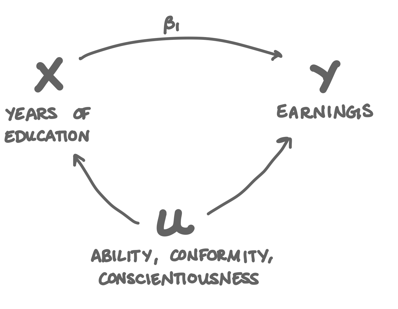
The field of Education Economics is concerned with, more than anything else, this regression:
\[\text{Earnings}_i = \beta_0 + \beta_1 \text{Education}_i + u_i\]
Take any dataset, around the world, throughout history, add as many other explanatory variables as you like (field, industry, gender, experience, parent’s education, etc) and you’ll find that the years someone spends in school seems to have an incredibly large and positive effect on their earnings down the road (\(\beta_1\) is large and very statistically significant). And that makes sense: education should give you the skills and the new ways of thinking that ensure you’ll be successful in the real world. If it didn’t, what would be the point?
The thing is, the size of that \(\hat{\beta}_1\) is so large and positive that you have to wonder: if education is such a good investment, why do so many people drop out of high school and college? As economists, we don’t usually like to chalk things up to irrational behavior. There has to be something else going on!
The answer: there’s omitted variable bias in that regression. The omitted variables: ability, conscientiousness, and conformity.
The solution: the Econometrician’s causal inference toolkit (instrumental variables, differences in differences, regression discontinuity, etc).
Questions
In the regression
earnings ~ education, we usually find:- A small, near-zero, and statistically insignificant \(\beta_1\): it looks like education has little to no effect on a person’s earnings down the road.
- A large, negative, and statistically significant \(\beta_1\): it looks like education reduces a person’s earnings down the road by a lot.
- A large, positive, and statistically significant \(\beta_1\): it looks like education boosts a person’s earnings down the road by a lot.
- A moderate, unstable, and statistically insignificant \(\beta_1\): it looks like the relationship between education and earnings is weak and inconsistent across samples.
If we estimate
earnings ~ educationand get a large and statistically significant \(\beta_1\), should we be suspicious?- Yes, because omitted variables like ability affect both education and earnings, so the estimate may be biased upward.
- No, because a large and statistically significant \(\beta_1\) shows a strong causal effect of education on earnings.
- No, because statistical significance means the estimate is accurate and not driven by other factors.
- Yes, because large coefficients are often caused by random variation in the data rather than real relationships.
In the regression
y ~ x, when does an omitted variableoconfound the relationship and lead to a biased estimate of \(\beta_1\)?- When
ois correlated withybut not correlated withx, you’ll always get omitted variable bias, no matter the sample size. - When
ois correlated withyand correlated withx, you’ll always get omitted variable bias, no matter the sample size. - When
ois correlated withxbut not correlated withy, you’ll always get omitted variable bias, no matter the sample size. - When
ois not correlated withynor withx, you’ll always get omitted variable bias, no matter the sample size.
- When
When can you interpret \(\beta_1\) as the causal effect of an explanatory variable \(x\) on the dependent variable \(y\)?
- When the regression includes many control variables, so most sources of bias have been accounted for.
- When there is no omitted variable bias: there is no variable \(o\) that is correlated with both \(x\) and \(y\).
- When \(\beta_1\) is statistically significant, so the relationship is unlikely to be due to chance.
- When the sample size is very large, so the estimate is precise and stable.
Suppose you’re studying how the number of opposite sex friends affects high school GPA, but you omit parental strictness. Will this add bias?
- Yes, because parental strictness affects both the number of opposite sex friends and GPA, so the estimate will be biased.
- No, because parental strictness only affects GPA and not the number of opposite sex friends.
- No, because the number of opposite sex friends is the main factor determining GPA.
- Yes, but only if parental strictness is measured with error in the data.
Consider the regression
weight_lost ~ gym_visits. Suppose you get a large, statistically significant estimate for \(\beta_1\). Should you report that going to the gym seems to cause people to lose weight?- Yes, because a large and statistically significant \(\beta_1\) shows that gym visits strongly increase weight loss.
- Yes, because gym visits occur before weight loss, so the direction of causality is clear.
- No, because omitted variables could affect both gym visits and weight loss, biasing the estimate.
- No, because weight loss is mostly random and cannot be explained by behaviors like gym visits.
What omitted variables should we be worried about to bias \(\beta_1\) in the regression
weight_lost ~ gym_visits?time_of_day: varies across gym visits but does not directly affect weight loss outcomes.gym_location: differs across individuals but is not related to weight loss behavior.diet_discipline: correlated with both gym visits and weight loss, so omitting it biases the estimate.music_played: may vary at the gym but does not influence weight loss or gym attendance decisions.
Download this assignment
Here’s a link to download this assignment.