library(tidyverse)10 Functional Programming with map()
By the end of this assignment, you should be able to:
- Explain what an anonymous function is and why we use it.
- Use
ggplot() + stat_function()with anonymous functions as a “graphing calculator.” - Use
map()to repeat a task many times and combine the results into a tibble. - Run an OLS simulation.
Run this code to attach the tidyverse to your current session and get started.
Anonymous Functions
An anonymous function is a function without a name. You write it when you want a quick “one-time” function.
# do not run

function(input) {
  # do something with input
}
Example: Apply a function immediately
This creates a function function(x) {3 * x} and immediately calls it with x = 9.
(function(x){3 * x})(9)[1] 27(Of course, if you want to know what 3 * 9 is, 3 * 9 is a much simpler way of solving the problem.)
Question 1
Write an anonymous function that divides any input by 3, and then call that function on the vector c(1, 3, 9).
R as a Graphing Calculator
You can graph functions with ggplot by using stat_function() paired with an anonymous function.
ggplot() +
  stat_function(fun = function(x) 2 * x + 1, color = "red")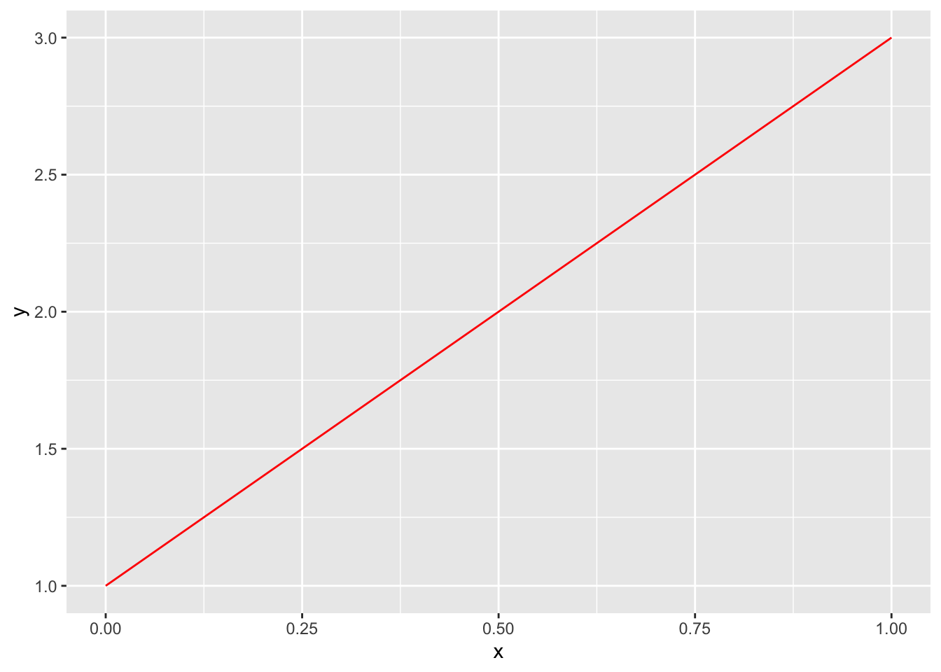
Zoom in or out using xlim() and ylim().
ggplot() +
  stat_function(fun = function(x) 2 * x + 1, color = "red") +
  xlim(0, 3) +
  ylim(0, 6)
Warning: Removed 17 rows containing missing values or values outside the scale range
(`geom_function()`).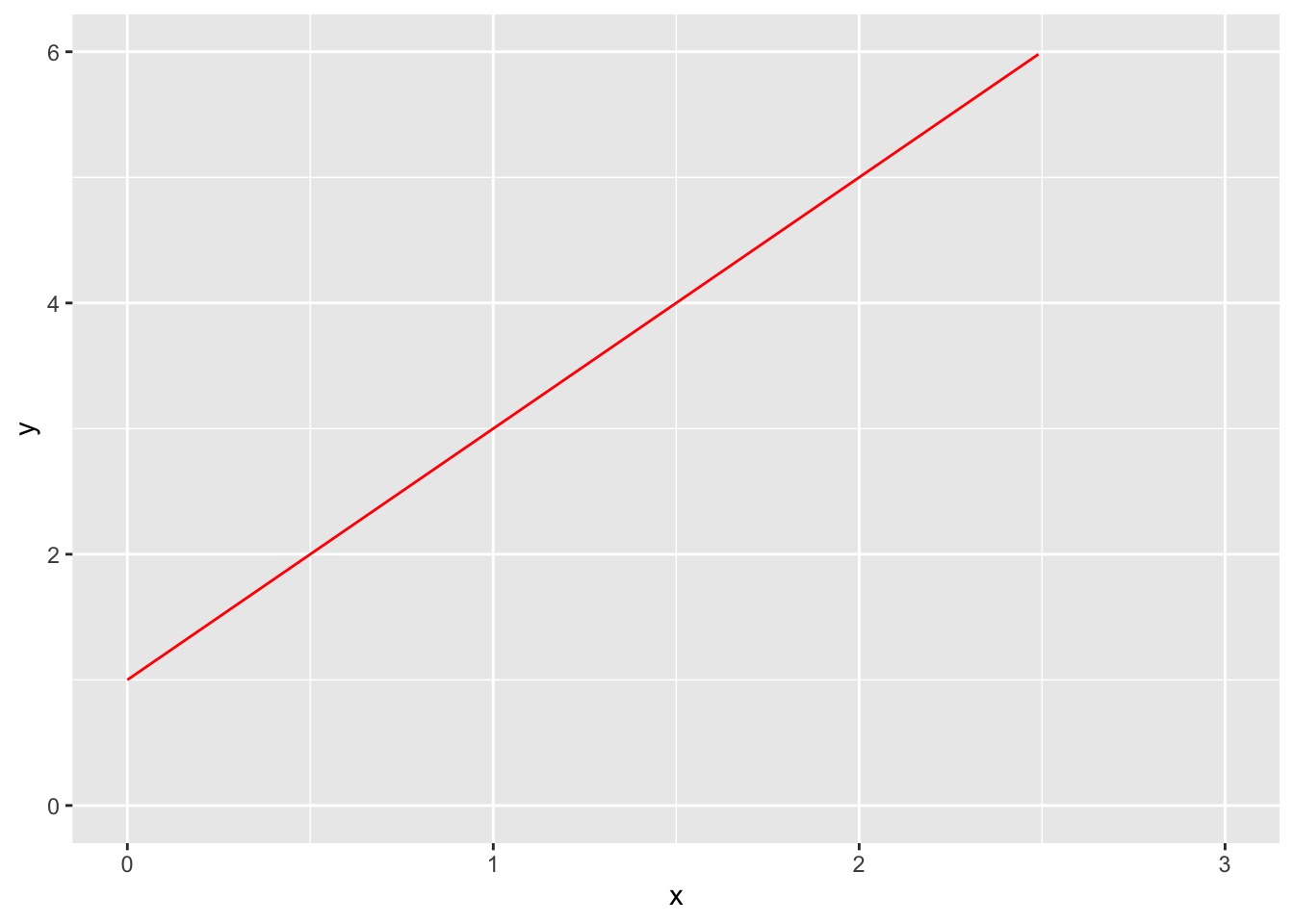
Question 2
Use ggplot to graph the function \(y = x^2 + 4x - 1\) in blue. Set x and y limits appropriately.
map() for a Simple Task
Why map()?
Sometimes you want to do the same task many times, once for each element of a list or vector. map() forms a mapping from the inputs to outputs, as defined by the anonymous function you use. map() takes two arguments:
.x: a list of inputs.f: the function you want to call on each element of those inputs.
# do not run
map(.x = <vector_or_list>, .f = <function>)
Example: square a bunch of numbers
A silly example: use map() to square every number from 1 to 5. .x is the vector 1:5; .f is a function that squares a number.
map(
  .x = 1:5,
  .f = function(number) {
    number^2
  }
)
[[1]]
[1] 1
[[2]]
[1] 4
[[3]]
[1] 9
[[4]]
[1] 16
[[5]]
[1] 25Notice that map() returns a list: similar to a vector, but much more flexible. Lists can be nested and lists can contain different data types (like a character string as one element and a number as the next). If you want to return a vector at the end, just pipe the result into as_vector().
The example above is silly because many operations, including the square, is vectorized in R. A much simpler way to do this task is just:
(1:5)^2[1] 1 4 9 16 25Question 3
Use map() to divide every number from 1 to 100 by 2. Make sure that the output is a vector.
Of course, division is also vectorized. So a much simpler way to do this is:
(1:100)/2 [1] 0.5 1.0 1.5 2.0 2.5 3.0 3.5 4.0 4.5 5.0 5.5 6.0 6.5 7.0 7.5
[16] 8.0 8.5 9.0 9.5 10.0 10.5 11.0 11.5 12.0 12.5 13.0 13.5 14.0 14.5 15.0
[31] 15.5 16.0 16.5 17.0 17.5 18.0 18.5 19.0 19.5 20.0 20.5 21.0 21.5 22.0 22.5
[46] 23.0 23.5 24.0 24.5 25.0 25.5 26.0 26.5 27.0 27.5 28.0 28.5 29.0 29.5 30.0
[61] 30.5 31.0 31.5 32.0 32.5 33.0 33.5 34.0 34.5 35.0 35.5 36.0 36.5 37.0 37.5
[76] 38.0 38.5 39.0 39.5 40.0 40.5 41.0 41.5 42.0 42.5 43.0 43.5 44.0 44.5 45.0
[91] 45.5 46.0 46.5 47.0 47.5 48.0 48.5 49.0 49.5 50.0map() OLS Simulation
Now we’ll explore a more useful way to use map(), on functions that are not vectorized.
Question 4
First, I’ll generate some random data using rnorm(), which generates random numbers from the normal distribution. It takes n (number of observations to generate), mean, and sd (standard deviation). My x is pure noise around a mean of 50, and y depends partially on x and partially on its own random noise (we’d call this “u” or epsilon in econometrics).
Read the code closely: what are the true values for \(\beta_0\) and \(\beta_1\)?
tibble(
      x = rnorm(n = 100, mean = 50, sd = 10),
      y = 50 + 5 * x + rnorm(n = 100, mean = 0, sd = 100)
    )
# A tibble: 100 × 2
x y
<dbl> <dbl>
1 46.4 371.
2 58.1 319.
3 56.2 196.
4 55.3 141.
5 54.0 290.
6 37.8 329.
7 51.7 58.6
8 53.3 480.
9 60.2 224.
10 43.7 267.
# ℹ 90 more rowsQuestion 5
Take my data set and pipe it into lm() to estimate the line of best fit. Observe: do you get estimates that are close to the true values for \(\beta_0\) and \(\beta_1\). Run the code several times: you’ll get new estimates because rnorm() keeps on generating random numbers.
# tibble(
#   ___
#     ) %>%
#   lm(___) %>%
#   broom::tidy()
Question 6
Now use map() to run your code above 100 times, recording the estimate for \(\beta_1\) each time. Let your .x be 1:100 so we run the simulation 100 times. Let your .f take as an input the variable s, but don’t do anything with s in the body of your function because we don’t want anything about the simulation to change each time we run it. Use slice() and select() to only save the estimate for \(\beta_1\). After map(), pipe the result into bind_rows() to return a tibble instead of a list.
# map(
#   .x = ___,
#   .f = function(s) {
#     tibble(
#       ___
#     ) %>%
#       lm(___) %>%
#       broom::tidy() %>%
#       slice(___) %>%
#       select(___)
#   }
# ) %>%
#   bind_rows()
Question 7
Copy-paste everything you did in question 6, and pipe the resulting tibble into a ggplot histogram to visualize the distribution of one variable: the distribution of \(\beta_1\) estimates you found.
Download this assignment
Here’s a link to download this assignment.